Recap
Previous section introduced Langevin Dynamics, a special diffusion process that aims to generate samples from a distribution $p (x)$ . It is defined as:
$d x_{t} = s (x_{t}) d t + 2 d W_{t},$
or equivalently
$d x_{t} = \frac{1}{2} s (x_{t}) d t + d W_{t},$
where $d W_{t}$ could be roughly treated as $d t ϵ$ , where $ϵ \sim N (0, 1)$ is a standard Gaussian random variable. $s (x) = \nabla_{x} lo g p (x)$ is the score function. The Langevin dynamics for $p (x)$ acts as an identity operation on the distribution, transforming samples from $p (x)$ into new samples from the same distribution.

In this section, we present the key processes of Denoising Diffusion Probabilistic Models (DDPMs):

Forward Diffusion Process: How DDPMs gradually corrupt an image into pure Gaussian noise
Backward Diffusion Process: How DDPMs generate images by gradually denoising pure Gaussian noise

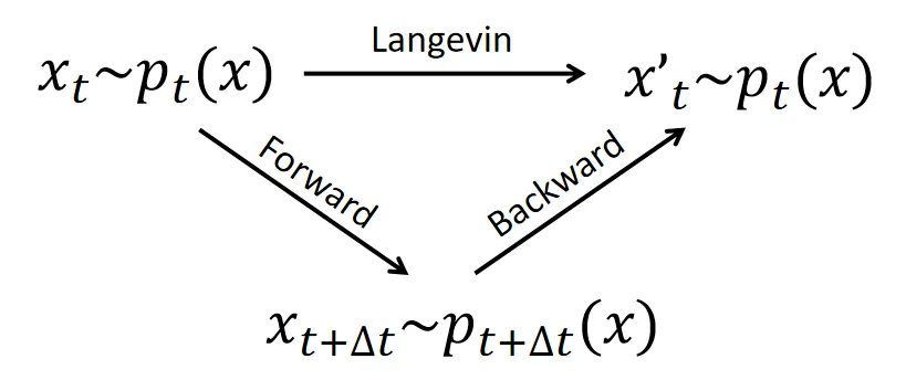
We will show how to derive the backward diffusion process from the forward process with the help of the triangle relation: foo

Prerequisites: Calculus, SDE and Langevin Dynamics.

Spliting the Identity: Forward and Backward Processes in DDPM#

The Denoising Diffusion Probabilistic Models (DDPMs) ¹ are models that generate high-quality images from noise via a sequence of denoising steps. Denoting images as random variable $x$ of the probabilistic density distribution $p (x)$ , the DDPM aims to learn a model distribution that mimics the image distribution $p (x)$ and draw samples from it. The training and sampling of the DDPM utilize two diffusion process: the forward and the backward diffusion process.

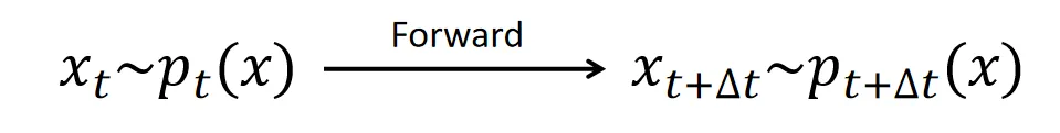
The Forward Diffusion Process#

The forward diffusion process in DDPM generates the necessary training data: clean images and their progressively noised counterparts. It gradually adds noise to existing images $x_{0} \sim p (x)$ using the Ornstein-Uhlenbeck diffusion process (OU process) ² within a finite time interval $t \in [0, T]$ . The OU process is defined by the stochastic differential equation (SDE):

d x_{t} = - \frac{1}{2} x_{t} d t + d W_{t},

in which $t$ is the forward time of the diffusion process, $x_{t}$ is the noise contaminated image at time $t$ , and $W_{t}$ is a Brownian noise.

Note that $- x$ is just the score function of the standard Gaussian distribution $N (0, I)$ . Thus, the forward diffusion process corresponds to the Langevin dynamics of the standard Gaussian $N (0, I)$ .

The forward diffusion process has $N (0, I)$ as its stationary distribution. This means, for any initial distribution $p_{0} (x)$ of positions ${x_{0}^{(1)}, ..., x_{0}^{(N)}}$ , their density $p_{t} (x)$ converges to $N (0, I)$ as $t \to \infty$ . When these positions represent vectors of clean images, the process describes a gradual noising operation that transforms clean images into Gaussian noise.

One forward diffusion step with a step size of $Δ t$ is displayed in the following picture. foo

The Backward Diffusion Process#

The backward diffusion process is the conjugate of the forward process. While the forward process evolves $p_{t} (x)$ toward $N (0, I)$ , the backward process reverses this evolution, restoring $N (0, I)$ to $p_{t}$ .

To derive it, we employ Langevin dynamics as a stepping stone, which provides a starightforward way to obtain the backward diffusion process:

NOTE
$Langevin Dynamics$ functions as an “identity” operation with respect to a distribution. Given that the backward process is the reverse of the forward process, the composition of the forward and backward process at time $t$ must therefore reproduce the Langevin dynamics for $p_{t} (x)$ , as shown in the following picture

To formalize this, consider the Langevin dynamics for $p_{t} (x)$ with a distinct time variable $τ$ , distinguished from the forward diffusion time $t$ . This dynamics can be decomposed into forward and backward components as follows:

d x_{τ} = s (x_{τ}, t) d τ + 2 d W_{τ}, = Forward - \frac{1}{2} x_{τ} d τ + d W_{τ}^{(1)} + Backward (\frac{1}{2} x_{τ} + s (x_{τ}, t)) d τ + d W_{τ}^{(2)},

where $s (x, t) = \nabla_{x} lo g p_{t} (x)$ is the score function of $p_{t} (x)$ . We have utilized the property that $2 d W_{τ} = 2 d t ϵ = d t ϵ_{1} + d t ϵ_{2} = d W_{τ}^{(1)} + d W_{τ}^{(2)}$ .

The “Forward” part in this decomposition corresponds to the forward diffusion process, effectively increasing the forward diffusion time $t$ by $d τ$ , bringing the distribution to $p_{t + d τ} (x)$ . Since the forward and backward components combine to form an “identity” operation, the “Backward” part must reverse the forward process—decreasing the forward diffusion time $t$ by $d τ$ and restoring the distribution back to $p_{t} (x)$ .

Now we can define the backward process according to the backward part in the equation above, and a backward diffusion time $t^{'}$ different from the forward diffusion time $t$ :

d x_{t^{'}} = (\frac{1}{2} x_{t^{'}} + s (x_{t^{'}}, t)) d t^{'} + d W_{t^{'}} .

One step of this backward diffusion process with $d t^{'} = Δ t$ acts as a reversal of the forward process. foo

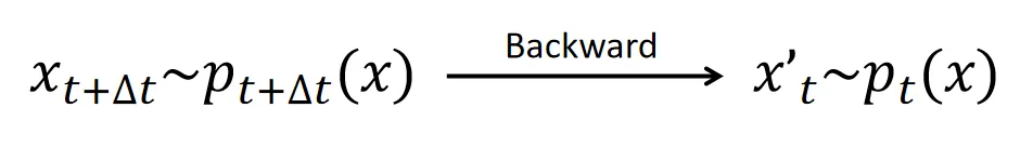
The backward diffusion process itself is also a standalone SDE that advances the backward diffusion time $t^{'}$ . If $x_{t^{'}} \sim q_{t^{'}} (x)$ , then one step of the backward diffusion process with $d t^{'} = Δ t^{'}$ brings it to $x_{t^{'} + Δ t^{'}} \sim q_{t^{'} + Δ t^{'}} (x)$ . foo

These two interpretations help us determine the relationship between the forward diffusion time $t$ and the backward diffusion time $t^{'}$ . Since $d t^{'}$ is interpreted as a “decrease” in the forward diffusion time $t$ , as well as a “increase” of the backward diffusion time $t^{'}$ , we have

d t = - d t^{'}

which means the backward diffusion time is the inverse of the forward. To make $t^{'}$ lies in the same range $[0, T]$ of the forward diffusion time, we define $t = T - t^{'}$ . In this notation, the backward diffusion process ³ is

d x_{t^{'}} = (\frac{1}{2} x_{t^{'}} + s (x_{t^{'}}, T - t^{'})) d t^{'} + d W_{t^{'}},

in which $t^{'} \in [0, T]$ is the backward time, $s (x, t) = \nabla_{x} lo g p_{t} (x)$ is the score function of the density of $x_{t}$ in the forward process.

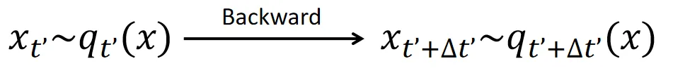
Forward-Backward Duality#

We have previously shown that a backward step is the reverse of a forward step: advancing time $t^{'}$ in the backward process corresponds to receding time $t$ by the same amount in the forward process. What then occurs when we chain together a series of forward and backward steps? Consider the following process: start with $x_{0}$ , evolve it via the $Forward Process$ to $x_{T}$ , then take $x_{T}$ as the initial position $x_{0^{'}}$ of the $Backward Process$ and evolve it to $x_{T^{'}}$ . This sequence is illustrated in the figure below. 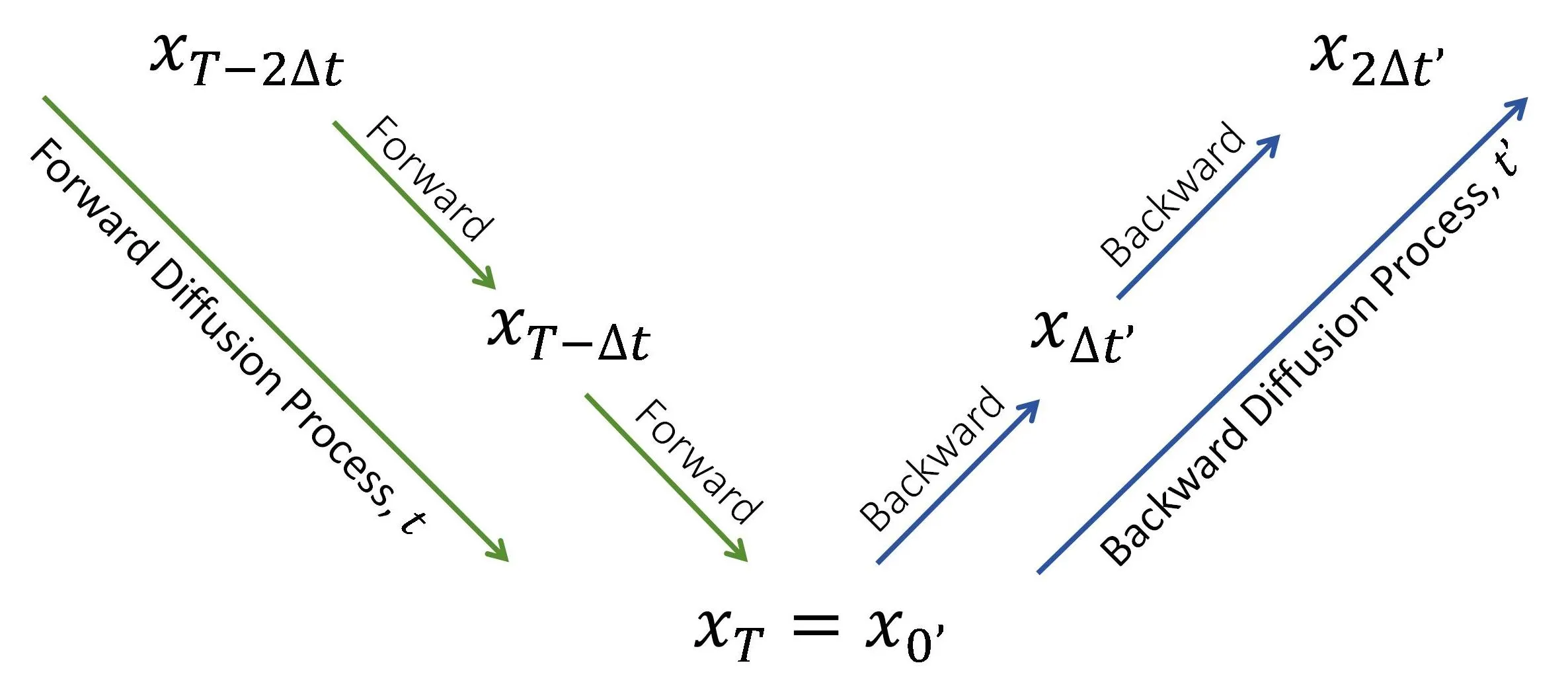foo The green arrows represent consecutive forward process steps that advance the forward diffusion time $t$ , while the blue arrows indicate consecutive backward process steps that advance the backward diffusion time $t^{'}$ .

We examine the relationship between $x_{t}$ in the forward diffusion process and $x_{t^{'} = T - t}$ in the backward diffusion process. The composition of a forward and a backward step constitutes a Langevin dynamics step. This allows us to connect $x$ in the forward process with those in the backward process through Langevin dynamics steps, as illustrated below: foo

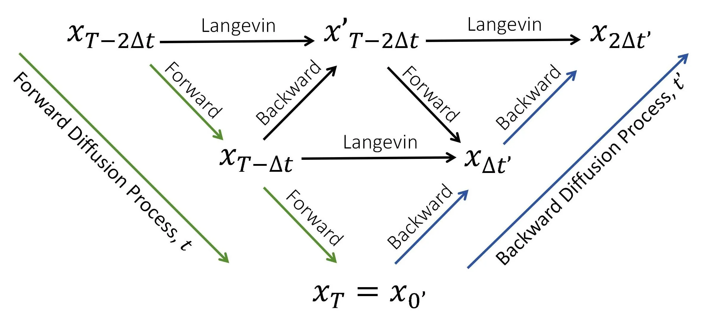
Each horizontal row in this picture corresponds to consecutive steps of Langevin dynamics, which alters the samples while maintaining the same probability density. This illustrates the duality between the forward and backward diffusion processes: while $x_{t}$ (forward) and $x_{(T - t)^{'}}$ (backward) are distinct samples, they obey the same probability distribution.

TIP
It’s important to note that the backward diffusion process does not generate identical samples to the forward process; rather, it produces samples according to the same probability distribution, due to the identity property of Langevin dynamics.

To formalize the duality, we define the densities of $x_{t}$ (forward) as $p_{t} (x)$ , the densities of $x_{t^{'}}$ (backward) as $q_{t^{'}} (x)$ . If we initialize

q_{0} (x) = p_{T} (x),

then their evolution are related by

q_{t^{'}} (x) = p_{T - t^{'}} (x)

For large $T$ , $p_{T} (x)$ converges to $N (x ∣ 0, I)$ . Thus, the backward process starts at $t^{'} = 0$ with $N (0, I)$ and, after evolving to $t^{'} = T$ , generates samples from the data distribution:

q_{T} (x) = p_{0} (x) (data distribution) .

This establishes an exact correspondence between the forward diffusion process and the backward diffusion process, indicating that the backward diffusion process can generate image data from pure Gaussian noise.

What is Next#

We demonstrated that backward diffusion—the dual of the forward process—can generate image data from noise. However, this requires access to the score function $s (x, t) = \nabla_{x} lo g p_{t} (x)$ at every timestep $t$ . In practice, we approximate this function using a neural network. In the next section, we will explain how to train such score networks.

Stay tuned for the next installment!

Discussion#

If you have questions, suggestions, or ideas to share, please visit the discussion post.

Cite this blog#

This blog is a reformulation of the appendix of the following paper.

1
@misc{zheng2025lanpainttrainingfreediffusioninpainting,
2
      title={LanPaint: Training-Free Diffusion Inpainting with Asymptotically Exact and Fast Conditional Sampling},
3
      author={Candi Zheng and Yuan Lan and Yang Wang},
4
      year={2025},
5
      eprint={2502.03491},
6
      archivePrefix={arXiv},
7
      primaryClass={eess.IV},
8
      url={https://arxiv.org/abs/2502.03491},
9
}

Ho, J., Jain, A., & Abbeel, P. (2020). Denoising diffusion probabilistic models. Advances in neural information processing systems, 33, 6840-6851. ↩
Uhlenbeck, G. E., & Ornstein, L. S. (1930). On the theory of the Brownian motion. Physical Review, 36(5), 823–841. ↩
Anderson, B. D. O. (1982). Reverse-time diffusion equation models. Stochastic Processes and their Applications, 12(3), 313–326. ↩

Spliting the Identity: Forward and Backward Processes in DDPM#

The Forward Diffusion Process#

The Backward Diffusion Process#

Forward-Backward Duality#

What is Next#

Discussion#

Cite this blog#

Footnotes#